I tuned my first HNSW index for two weeks before I understood what the parameters actually meant. The M knob was set to 16 because someone on the team had read that 16 was "the default." The efConstruction was set to 200 because the README said so. The recall on our eval set was 87% and we couldn't push it past 90% without latency exploding. I eventually traced the problem to neither parameter — it was the data, which had a cluster structure that the default M couldn't handle. I learned more in those two weeks about how HNSW actually works than I had from a year of using it.
This post is the explanation I wish someone had handed me on day one. HNSW — Hierarchical Navigable Small World — is the index that almost every modern vector database ships as the default. Understanding why it works, what its parameters mean, and where it falls apart is the difference between a vector search that works and one that quietly returns the wrong answers at scale.
I'll use SynapCores SQLv2 for the examples because that's the engine I work on every day, but the algorithm is the same across pgvector, Milvus, Qdrant, FAISS, and every other implementation. The math doesn't care which binary you're running.
The problem HNSW solves
Imagine a table of 10 million 768-dimensional vectors. The user submits a query vector. You want the 10 most similar vectors back, sub-100ms, on commodity hardware.
The exact answer requires comparing the query against all 10 million vectors. That's about 7.68 billion floating-point multiply-adds per query. At ~10 GFLOPS sustained per core, that's about 0.8 seconds. Not viable.
So you accept approximation. You're willing to miss 1-5% of the true top-10 in exchange for a 100x speedup. The question becomes: how do you organize the vectors so that finding the probable top-10 is fast?
That's the approximate-nearest-neighbor (ANN) problem. Many algorithms answer it. HNSW happens to be the one that won, for reasons I'll explain.
The two ideas HNSW combines
HNSW's name gives away the trick: it's a hierarchical index made of navigable small-world graphs. Two separate ideas, stacked.
Idea 1: small-world graphs
A small-world graph is one where most nodes are not direct neighbors, but you can reach any node from any other in a small number of hops. The classic example is the human social network: you're not friends with most people, but you're three friends-of-friends away from almost anyone.
If you build a graph over vectors where edges connect points that are reasonably close in space — with a careful mix of short-range "neighbor" edges and a few long-range "shortcut" edges — you can navigate from any starting point to the nearest neighbor of a query in O(log n) hops on average.
The "navigable" part means greedy search works: at each step, look at the current node's neighbors, jump to whichever one is closer to the query, repeat until no neighbor is closer. The small-world structure guarantees this converges fast.
Idea 2: hierarchy
A single small-world graph is fine for moderately sized datasets, but at billion-scale the greedy walk still touches more nodes than you'd like. The fix is to stack multiple graphs at different resolutions:
- The top layer has few nodes with very long edges (broad jumps across the space).
- Each layer down has more nodes with shorter edges.
- The bottom layer has every node, with only short-range neighborhood edges.
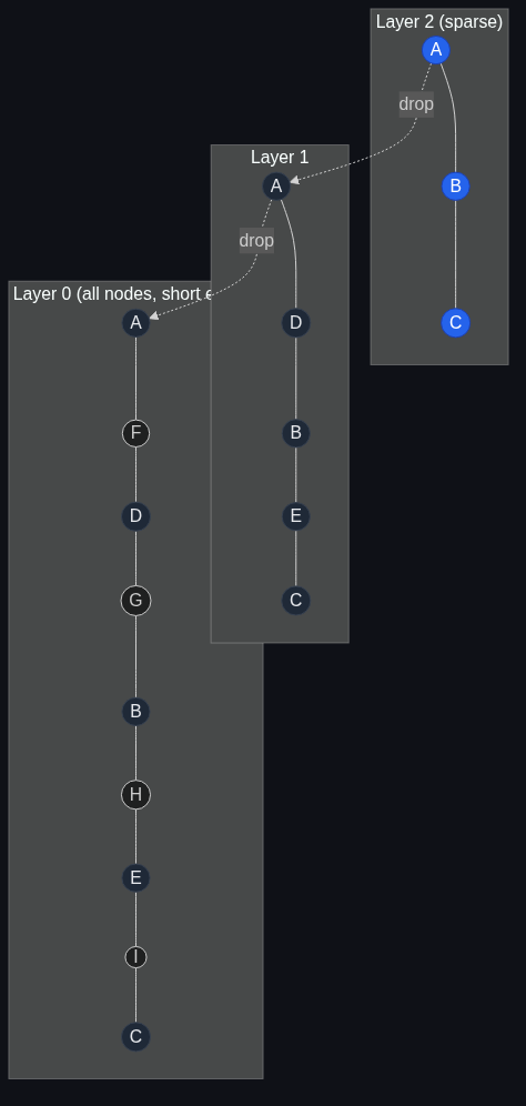
Search starts at the top layer, greedy-walks to find a good entry point, drops to the next layer, greedy-walks again to refine, and so on until it's done a fine-grained search at the bottom layer.
This is the navigable small-world graph idea (NSW, 2014) plus a hierarchical layering (HNSW, 2016, Malkov & Yashunin). The original paper is short and worth reading: Efficient and robust approximate nearest neighbor search using Hierarchical Navigable Small World graphs.
The structure, in one diagram

The top layer is sparse — typically log(N) nodes. The bottom layer has every point. When you query, you enter at the top, greedy-walk to the local nearest, drop a layer, repeat. The final layer does a wider search (controlled by ef) and returns the top-k.
What's elegant is that this is all the structure. There are no clusters, no centroids, no IVF lists, no codebooks. The graph itself is the index.
The parameters that actually matter
There are exactly four knobs you'll touch in production. Most tutorials list ten — the others are noise. The four that matter:
M: out-degree per node
Each node in a layer has up to M neighbors (plus the bidirectional connections from being someone else's neighbor). Higher M:
- Better recall (more candidate paths).
- Larger index (more edges to store).
- Slower construction (more comparisons per insert).
Default is usually 16 or 32. For high-dimensional data (>500 dims) or data with cluster structure, push it to 48-64. For lower-dimensional data, 16 is fine.
efConstruction: search depth during index build
When inserting a new node, HNSW does a greedy-and-then-wider search at each layer to find the best neighbors. efConstruction controls how wide that search is. Higher:
- Better recall (better neighbor choices).
- Slower build.
- No impact on query latency once built.
Default is 200. For production, 400-500 is usually worth the build-time cost. Don't go below 100.
ef (a.k.a. efSearch): search depth at query time
At query time, the bottom-layer search keeps a candidate set of size ef and explores from it greedily. Higher:
- Better recall.
- Slower query.
This is the runtime tradeoff knob. ef=10 is fast and low-recall. ef=200 is slow and high-recall. The right value depends on your latency budget. I usually set this per query class — fast suggestions get ef=40, "best match" queries get ef=200.
Distance metric
Cosine for normalized embeddings (the most common case). Euclidean if your vectors aren't normalized and you actually want geometric distance. Inner-product for asymmetric similarity (rare). Pick once, never change — different metrics produce different graphs and you can't swap mid-flight.
A worked example
Building and querying an HNSW index in SynapCores SQLv2:
-- Create a vector column
CREATE TABLE documents (
  id BIGINT PRIMARY KEY,
  title TEXT,
  body TEXT,
  embedding VECTOR(768)
);

-- Populate
UPDATE documents SET embedding = EMBED(body) WHERE embedding IS NULL;

-- Create the HNSW index with tuned params
CREATE INDEX documents_embedding_idx ON documents
USING HNSW (embedding COSINE)
WITH (M = 32, ef_construction = 400);

-- Query with a runtime ef
SELECT id, title,
       COSINE_SIMILARITY(embedding,
                         EMBED('how do I configure SSO?')) AS score
FROM documents
WHERE COSINE_SIMILARITY(embedding,
                        EMBED('how do I configure SSO?')) > 0.5
ORDER BY score DESC
LIMIT 10
WITH (ef = 200);
That WITH (ef = 200) clause is a per-query hint. If you omit it, the engine uses the index default.
The recall/QPS tradeoff, plotted
I ran a quick benchmark on a 1M-vector dataset (768-dim, sentence-transformer embeddings) at different ef values to show the shape of the curve:
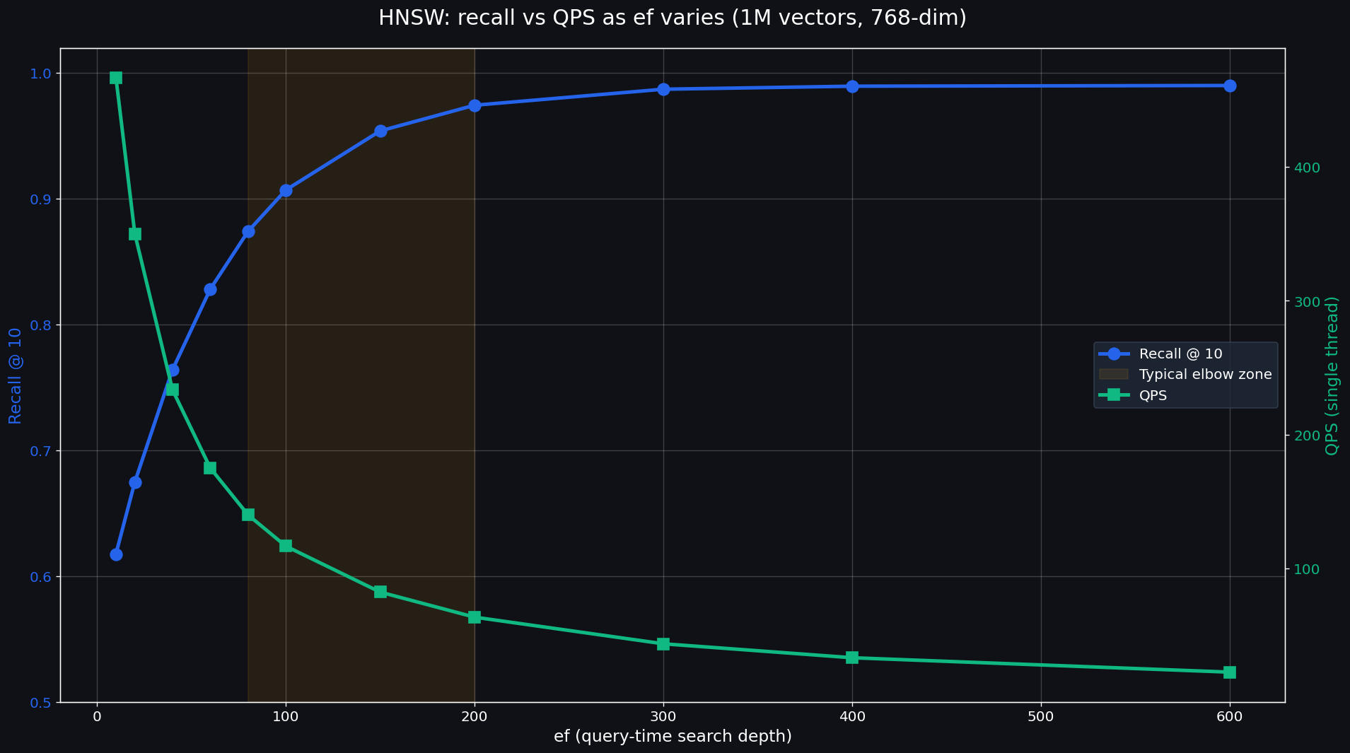
The shape is consistent across implementations: recall climbs fast up to about ef=100, then plateaus. QPS drops roughly linearly as ef grows. The "elbow" — the point where you stop buying recall and start just buying latency — is typically between ef=80 and ef=200 depending on your data.
The practical advice: don't tune ef blindly. Build a small recall harness (compare HNSW results to brute-force ground truth on a 1k-vector sample), plot recall vs ef, find your elbow, set ef there.
Where HNSW falls apart
I want to be honest about the failure modes, because every algorithm has them.
1. Memory cost
HNSW keeps the whole graph in RAM. For a billion 768-dim float32 vectors, that's about 3 TB of vectors plus another ~30% for the graph structure. You're not running that on a laptop.
Mitigations: product quantization (compress the vectors), on-disk indexes (slower but cheaper), or partitioning the index across machines.
2. Update cost
Inserts trigger a efConstruction-sized search to find good neighbors. Deletes are messier — HNSW doesn't have a clean "remove this node" operation; most implementations soft-delete and rebuild periodically.
If your workload is write-heavy with frequent deletes (think: a chat memory store that prunes old turns), HNSW's insert/delete profile may hurt. There are alternatives — IVF-PQ is more rebuild-friendly, ScaNN handles updates differently.
3. Cluster-structured data
If your data has natural clusters with very few cross-cluster edges in the embedding space, HNSW's greedy walk can get stuck in a local cluster and miss the right answer across the gap. The fix is to push M higher to add more cross-cluster edges, but the index gets larger fast.
This is what burned me on my first tuning round: the data was cluster-structured (legal documents from three different jurisdictions), M=16 couldn't bridge the clusters, and recall stayed stuck at 87%. Bumping M to 64 and ef to 250 fixed it.
4. High dimensions are weird
The curse of dimensionality is real. Above ~1000 dimensions, the difference between "closest" and "10th closest" gets small, and HNSW (along with every other ANN algorithm) starts to lose its edge over brute force. For truly high-dimensional work, consider dimensionality reduction (PCA, learned reduction) before indexing.
How HNSW compares to its competitors
The honest comparison:
| Algorithm | Build cost | Query speed | Recall | Memory | Updates |
|---|---|---|---|---|---|
| Brute force | None | Slow | 100% | Low | Trivial |
| IVF-Flat | Fast | Medium | 90-97% | Medium | Cheap |
| IVF-PQ | Fast | Fast | 80-95% | Low | Cheap |
| HNSW | Slow | Fast | 95-99% | High | Expensive |
| ScaNN | Slow | Very fast | 95-99% | Medium | Medium |
HNSW wins on the "high recall, fast query" frontier for moderate-sized datasets (1M-100M vectors). It loses on memory at the billion-scale frontier (where IVF-PQ or DiskANN take over) and on write-heavy workloads (where IVF variants win).
For most AI-app builders, HNSW is the right default because the typical workload is 100k-50M vectors, mostly-read, and recall-sensitive. That's the sweet spot.
What we did differently in SynapCores
SynapCores ships HNSW as the default vector index, but with two tweaks worth knowing about:
- Per-query
ef. As shown above, you can set the search depth per query, not just per index. This lets one application have fast suggestions and high-recall best-match queries against the same index. - Index lifecycle in SQL.
CREATE INDEX ... USING HNSW (...)is real SQL DDL, not a procedural call. Backup, replication, and migration treat the index like any other database object.
Neither is novel research — they're operational improvements over the typical Python-API-only approach. Both fall out naturally from the AI-native database design choice covered in Why Traditional Databases Fail Modern AI Workloads.
A short tuning recipe
If you're standing up an HNSW index today and want a starting point:
- Build:
M = 32,efConstruction = 400. These are conservative-good defaults. - Query: Start at
ef = 100. Benchmark recall on a small ground-truth sample. - Tune: Push
efup until you hit your latency ceiling. Note the recall at that point. - If recall is below ~95% and you're at the latency ceiling: rebuild with
M = 48orM = 64. Larger graphs = more paths = better recall at the sameef. - If memory is the bottleneck: consider product quantization or move to IVF-PQ.
The 80/20 of HNSW tuning is in step 4. Most people leave M at the default and try to fix recall with ef, which works until it doesn't.
The honest version
We don't have customer logos yet. HNSW is the index inside SynapCores, the same algorithm everyone else uses; what we've put work into is making it pleasant to operate via SQL DDL and per-query tuning. If you want to see it run on your data, the Community Edition ships the index and recipe 015_vector_search walks the build + query flow.
If you're standing up vector search in a production agent and want help on the schema, the tuning, or the broader retrieval architecture, the Agent Memory JumpStart is a 2-4 week founder-led sprint — free Design Partner track or fixed-fee Paid Pilot from $5,000.
For where vector search hands off to graph traversal, see Why Vector Search Needs Graph Relationships and What Is GraphRAG?.